Modeling Swiss Toponyms with NLP
TLDR In this post I teach a neural network the linguistic and geographical patterns of Swiss place names (‘toponyms’). The resulting model is able to generate new place names for a given location, predict the most likely location of an arbitrary (and potentially fictional) place name, and allows us to explore the geographic patterns underlying the distribution of Swiss place names.
Introduction
Thanks to its high population density and multilingual history, Switzerland features an amazing variety of geographic place names (or ‘toponyms’) in a fairly small area. I’ve often wondered about the logic underlying this distribution. Intuitively, I always felt like there were clear patterns, even within the four Swiss linguistic areas. A lot of places around Zürich seem feature the suffix ‘-ikon’, whereas places further West seem to end in ‘-igen’. Then again, we tend to see patterns where there aren’t any, so perhaps I’m wildly overestimating my geographic intuition.
In this project, I’ll look at Swiss place names a bit more systematically, and will try to test my hypothesis that the geographic distribution of Swiss toponyms follows learnable patterns. Specifically, I’ll turn this into an NLP project and will try to answer the following questions:
- Can we determine the most likely location of a place name using only its morphology?
- Can we generate new place names that fit local morphological patterns?
- Which regions have similar place names, and which don’t? Where do the borders run through?
Data
The primary data source I use for this project is the Swissnames dataset published by the Swiss Federal Office for Topography (swisstopo). Specifically, I use the Swissnames polygon dataset containing information about populated places, district borders, public buildings (e.g. airports), and other named areas.
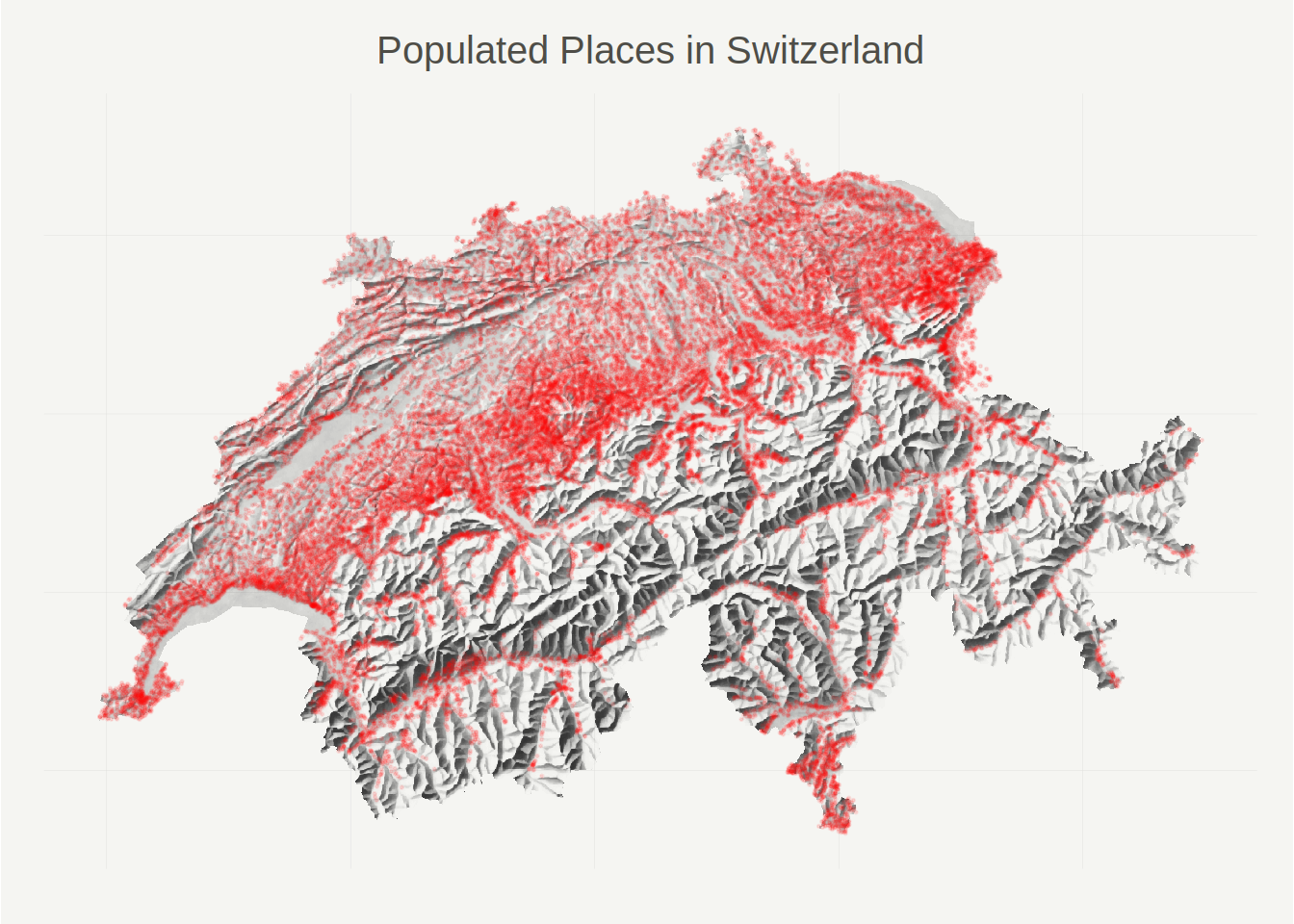
For this project, I focus exclusively on populated places. Prior to modeling, I preprocess the data in multiple steps. I clean the place names by removing punctuation characters (like dots and ampersands), replacing rare characters (e.g. “ì” with “i”), and deleting redundant white spaces. I also transform all text to lower case, and exclude duplicates and overly long place names (those with more than 16 characters). Further, I simplify the geographic part of the dataset by associating each populated place with a single coordinate (the centroid of its original polygon). After preprocessing, I end up with a bit more than 33.5k place names; note that many of these places are not official municipalities, but neighborhoods, hamlets, districts, etc. The following map plots the data, with each red dot representing a populated place.
A probabilistic ML approach
First, some rough definitions.
In the following, I use the term ‘location’ to refer to a specific point (or area) in (geographic) space, i.e. something you can describe with geographic coordinates. In contrast, when I use the term ‘(place) name’, I refer purely to a toponym (e.g. ‘Bern’), not the geographic location that toponym is commonly associated with (e.g., for the case of Bern, 46.9480° N, 7.4474° E). When I use the term ‘observations’, I mean observed (real-life) location-name pairs. Finally, where it helps the discussion, I use capitalized words to describe random variables (e.g. \(Pr(Location = x)\)), and lowercased words to describe realizations (e.g. \(location_i\)).
Now, let’s try to put our research questions from above into probabilistic language; this will help with formulating our NLP model later on. My first question was: Can we determine the most likely location of a place name using only its morphology? Here we’re asking for \(argmax_i \ Pr(Location = location_i \ | \ Name = name)\), the location (indexed by \(i\)) that is most likely to be attached to an observation with the toponym \(name\).
My second question was: Can we generate new place names that fit local morphological patterns? Here we’re simply asking to sample from the distribution \(Pr(name \ | \ location)\).
Third: Which regions have similar place names, and which don’t? Where do the borders run through? This one is a bit tougher. I’m going to go into more detail below, but essentially we can interpret this question as asking: What locations feature similar \(Pr(name \ | \ location)\) distributions? Between which locations does the conditional distribution \(Pr(name \ | \ location)\) change most quickly?
In summary, what we want are empirical estimates for the two conditionals \(Pr(location \ | \ name)\) and \(Pr(name \ | \ location)\). There are many ways we could address this. For reasons that I will address below, I will take the following approach:
- Build a character-level sequential model for \(Pr(name \ | \ location)\).
- Use the above model and some simple probability theory to estimate \(Pr(location \ | \ name)\).
A character-level RNN for toponyms
Our first goal will be learning \(Pr(name \ | \ location)\). To do so, I will rely on a character-level formulation of the problem, where I model toponyms as sequences of categorical random variables, each representing a single character (like ‘a’, ‘r’, or the space character). More formally, instead of treating place names as realiziations of a single categorical \(Name\) variable, I treat place names as realizations of a random vector \([X_1, X_2, \ldots, X_K]\), where each \(X_l\) is a categorical random variable with support over the letters of the German, French, and Italian alphabets. To ensure that we can model all place names in our dataset with a random vector of uniform length, I extend all place names to 16 characters by padding with the space character as necessary.
The character-level approach allows us to factorize \(Pr(name \ | \ location)\) into a product of conditional distributions, specifically
\[ \begin{align} Pr(name \ | \ location) = & \phantom{*} Pr(x_1 \ | \ location) \\ & * Pr(x_2 \ | \ location, x_1) \\ & \ldots \\ & * Pr(x_{16} \ | \ location, x_1, x_2, \ldots, x_{15}). \end{align} \]
This factorization has two key benefits: First, we only need to model PMFs with support of size \(39\) (the number of distinct characters in our place names), instead of \(39^{16}\) (the whole space of possible words). Second, sampling new place names is simple because we can iteratively sample from the conditionals. This is also the primary reason I build a model for \(Pr(name \ | \ location)\) instead of the (potentially simpler) \(Pr(location \ | \ name)\). The latter model would not be amenable to sampling place names.
At this point, all we need is a way to learn the \(Pr(x_t \ | \ location, x_{1:{t-1}})\) conditionals. I use a GRU RNN for this task. RNNs (recurrent neural networks) are neural networks designed to process sequences. In contrast to their more widely known cousin, the feed-forward neural net, RNNs are stateful. Specifically, predictions in RNNs are a function of the state at step \(t\), \(h_t\), which in turn is a function of both the features passed to the network at step \(t\), as well as \(h_{t-1}\); this way, features passed to the RNN at steps prior to \(t\) are allowed to affect the prediction at step \(t\) through the state. If you’d like to learn more about RNNs, I think this blog post by Andrej Karpathy is pretty much required reading by now. Andrej also explains character-level RNNs in more detail than I do here.
A GRU (gated recurrent unit) is a RNN with a particular architecture. Putting it simply, a GRU is a RNN that learns what pieces of information are valuable to remember (and keep in the state), and what pieces of information can (and should) be forgotten. If you’d like to read more, I have found this article a useful starting point to learn about GRUs.
RNNs provide a very elegant modeling tool for our problem of learning \(Pr(x_t \ | \ location, x_{1:{t-1}})\). Instead of having to build a model that takes a varying number of previous characters (and some coordinate information) as input, RNNs permit modeling the conditional probabilities simply as \(Pr(x_t \ | \ h_t)\), where the state \(h_t\) encapsulates all relevant information about previous characters and the geographic location for which a prediction is being made. More specifically, I implement an RNN where the initial state is a (learned) function of the location for which a place name distribution is requested, and the ‘feature’ at step \(t\) is the character observed at step \(t-1\). To be slightly more formal, my modeling architecture is
\[ \begin{aligned} Pr(x_t \ | \ x_{1:{t-1}}, location) & = {softmax}(f_1(h_t, w_{f1})) \\ h_t &= g(h_{t-1}, x_{t-1}, w_g) \\ h_0 &= f_2({location}, w_{f2}) \end{aligned} \]
where \(g\) is a function representing a (triple stacked) GRU architecture and \(f_k\) are multilayer perceptrons. \(w_k\) are sets of learned weights. If you want all the nitty gritty details details, you can take a look at the R model implementation, and for details on training, see the training script.
Some first results: Generating new place names
We can now use our fitted RNN to have some fun and address our second question: Can we generate new place names that fit local morphological patterns? Or, more simply, can we generate new, realistically sounding Swiss place names? The way we do this is simple:
- Select some coordinates for which we want to sample place names.
- Pass those coordinates and some arbitrary ‘seeding’ character (representing \(x_1\), the first character in the sequence), to the RNN, yielding a distribution for \(x_2\).
- Sample \(x_2\) from that distribution.
- Feed \(x_2\) to the RNN, yielding a distribution for \(x_3\). Go to step 3. and repeat until 16 characters have been sampled.
Let’s start by sampling some place names for the coordinates of Zürich. In other words, we generate some toponyms that the model thinks are ‘typical’ for the coordinates at which Zürich happens to be located. We sample the seed characters randomly from the alphabet.
##  [1] "kaltersberghof" "im gross bechi" "baumen"         "engelbach"
##  [5] "rütingen"       "chrächlisrain"  "pfaffengasse"   "längenberg"
##  [9] "unter runten"   "widhalde"       "mungert"        "pfausenacker"
## [13] "inner katz"     "bommerthalden"  "mittel aesch"
While two of these refer to places that actually exist (‘Baumen’, ‘Längenberg’), all others were dreamt up by the model. Amazingly, to me as a Swiss German speaker, most of these actually sound like they could be places around Zürich. (Side note: if I had unlimited resources, I’d probably try to validate my model by evaluating the share of sampled names an average Swiss German speaker is able to identify as fake).
Next, let’s do the same thing for some other well-known places in Switzlerand. The following table shows 10 newly generated place names for each of the 6 towns listed in the column headers.
| lausanne | neuchâtel | interlaken | luzern | lugano | st moritz |
|---|---|---|---|---|---|
| krande la mâche | häuse | brucken | schweigibach | devera | calva |
| issinges | im chres les mon | chutze | eigeren | tarteta | löss |
| bergeret | oberts les aux m | bürstli | guggenbach | morcello | latgota |
| en prayert | champnet | brüggli | därtischwand | lorenta | sciola |
| ranccavaz | pré varot | tobleten | brüggelen | krarano | larova |
| champ coléche | berges | tännli | lüscher | bolere | wassalp |
| pré noun | en de branchen | hinterbühl | ried | caragnio | dala |
| la combe reande | undert dels | hinter eich | mittler stägert | stogno | grando |
| un de les bardes | sur la courette | lättihof | maurnisberg | davanti | longera |
| wauches | hintere herra | fossboden | aug dorf | sa cra | zereschg |
The model nicely adapts the samples to the different language regions; to my ear, the samples for Lausanne and Neuchâtel sound (mostly) French, the ones for Interlaken and Luzern sound (Swiss) German, the ones for Lugano Italian, and the ones for St. Moritz Romansh. Only about 7% of these samples are toponyms that actually exist (or, rather, that are in the dataset I used for training), all others were dreamt up by the model.
Because RNNs can process sequences of arbitrary length, we can also pass ‘seed’ strings consisting of more than one character to the model. Let’s see what happens if I generate toponyums using the first four letters of my own name (‘Phil’), paired with the same 6 locations used above:
| lausanne | neuchâtel | interlaken | luzern | lugano | st moritz |
|---|---|---|---|---|---|
| philon | philard | phileten | philberg | philo | phila |
| philcoux | philly | philfbach | philchhof | philz | phila |
| philles | phillarbin | philchingen | philkschhälderdi | philletto | philla |
| phile de liete | philerie | phillibach | phillingen | philstel | philadiva |
| phillon sux mèle | phila rot | philangischhubel | philki | philo | phila brugagl |
Personally, I like ‘Philadiva’ the most.
Finally, because it’s fun (and because I spent some time there), let’s see what happens if we turn Boston into a Swiss village…
| lausanne | neuchâtel | interlaken | luzern | lugano | st moritz |
|---|---|---|---|---|---|
| bostondes | bostonnraine mon | bostonihüsli | boston | bostone | bostona |
| bostont | boston frés novr | boston | boston | bostone | bostoni |
| bostonnens | boston | bostonimatt | bostonimatt | boston a | boston |
| boston | boston neuves | boston im see | boston | bostoni | boston |
| boston | bostonnet | boston | boston | bostonica | boston |
Can’t wait to eat some Lobster in ‘Boston im See’ (literally ‘Boston in the lake’)!
Some Bayesian trickery
At this point, we can try to address our initial question of whether it’s possible to determine the most likely location of a place name using only its morphology. More formally, we now want an estimate for \(Pr(location | name)\).
Fortunately, it’s relatively easy to do this using the RNN from above and some basic statistical theory. We start by noting that by applying Bayes theorem, we can write
\[ \begin{align} Pr(location | name) = \frac{Pr(name | location) Pr(location)}{Pr(name)}. \end{align} \]
This expression contains two unknown terms: The prior probability of observing a name, \(Pr(name)\), and the prior probability of observing a location \(Pr(location)\). We could come up with procedures to estimate these quantities, but they would be costly to implement, requring us to fit new models (for \(Pr(location)\)) and implement some numerical integration algorithm (for \(Pr(name)\)). Instead, I take a much simpler approach and assume that there are a finite number of coordinates at which a populated place may be located. Specifically, I focus on the centroid coordinates of the productive areas of the 2324 Swiss municipalities (as of 2015), as enumerated in this dataset distributed by Timo Grossenbacher (who’s also authored some of the beautiful map templates I’m using in this post). I also assume a uniform distribution for \(Pr(location)\), meaning I assume that prior to observing its associated toponym, any of the 2324 municipalities is equally likely to contain a given observations.
Now let’s call the center coordinate of the \(i\)th municipality \(coord_i\), and let \(Pr(name \ | \ Location = location_i) = r(name, coord_i)\) be the probability of observing a name at coordinate \(coord_i\) as estimated with the RNN introduced above. Then, we can write the probability of a certain name being located in municipality \(i\) as
\[ \begin{align} Pr(location = i | name) &= \frac{r(name, coord_i)}{Z_{name}} \\ Z_{name} & = \sum_i^N r(name, coord_i). \end{align} \]
which we can easiliy compute.
Some more results: Predicting locations
Equipped with the above expression, let’s have a look at some predictions. We’ll start by ‘predicting’ the location of ‘Zwinglikon’ - an imaginary place name constructed from ‘Zwingli’ (the famous protestant reformer from Zürich) and the suffix ‘-ikon’, which is typical for place names around Zürich and apparently has allemanic roots.
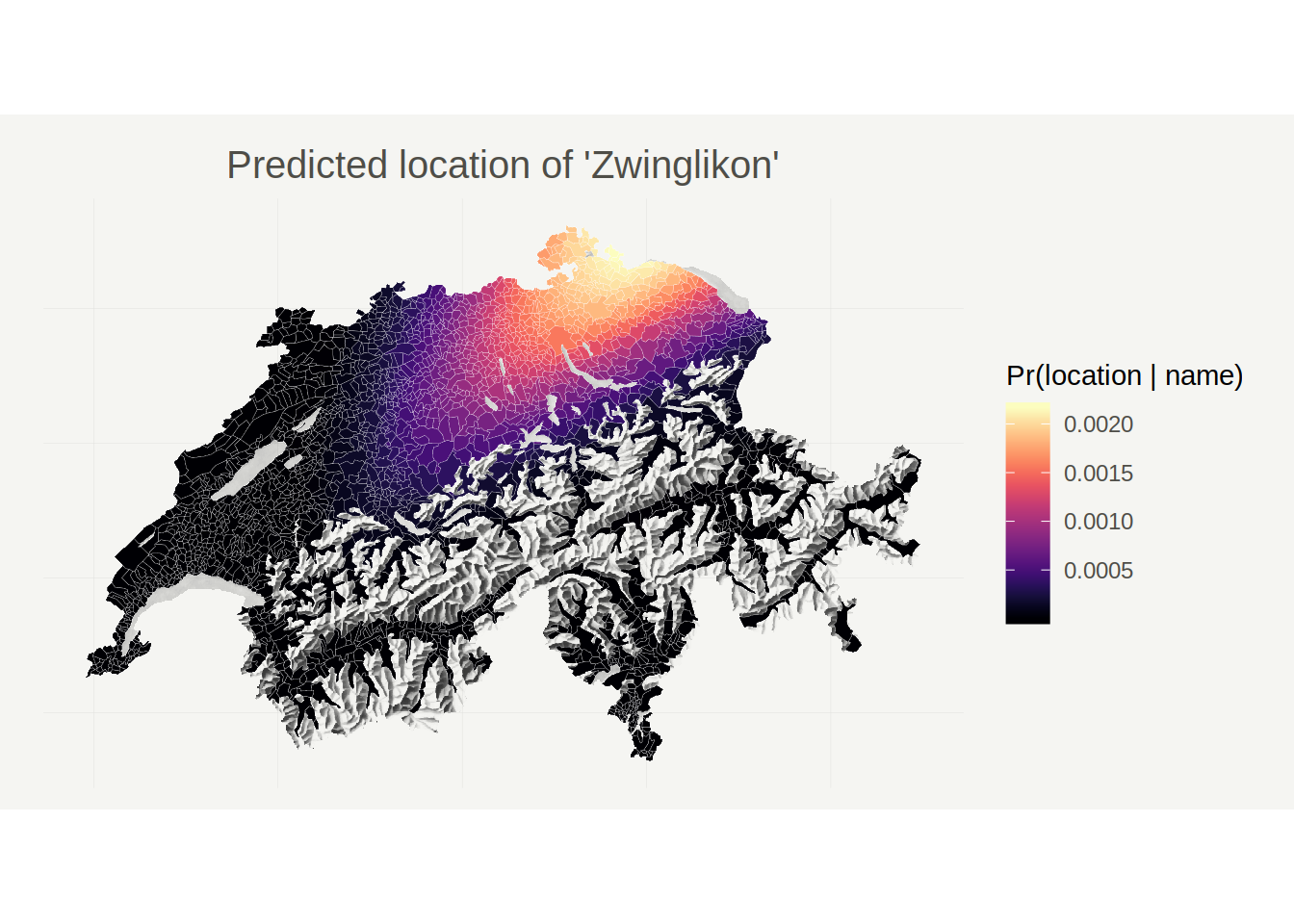
The map above shows each municipality’s predicted probability of containing a place named ‘Zwinglikon’. According to my model, ‘Zwinglikon’ would most likely be located somewhere between Schaffhausen, St. Gallen, and Zürich, which sounds pretty reasonable to me.
In the Introduction I hypothesized that the suffix ‘-igen’ is more common in toponyms to the West of Zürich. Let’s check whether the model agrees with me on that one and predict the location of ‘Zwingligen’.
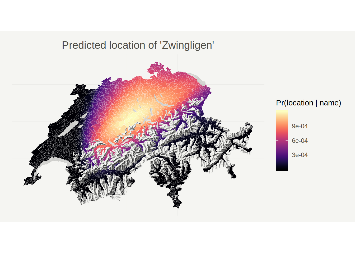
Indeed, it looks like ‘Zwingligen’ would be located closer to Bern than ‘Zwinglikon’.
Next, let’s see where my model would place ‘Milano’…
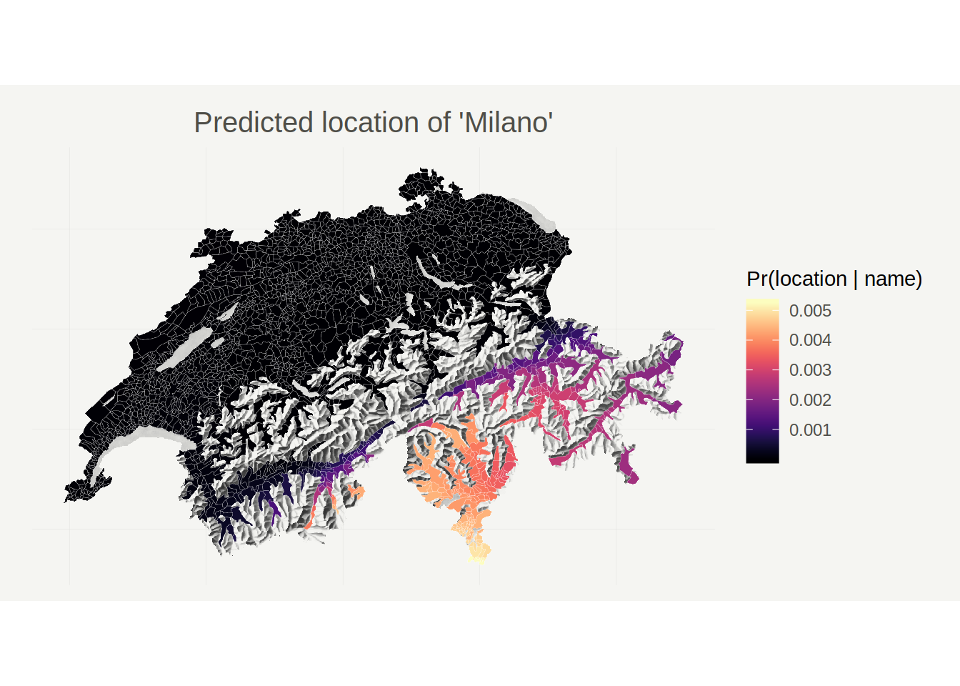
Unsurprisingly, if Milan were a city in Switzerland, it would most likely be located in the very South of the canton of Ticino (which, incidentally, is the place in Switzerland that’s geographically closest to the actual Milano).
Next, let’s try the same with a French city, Marseille.
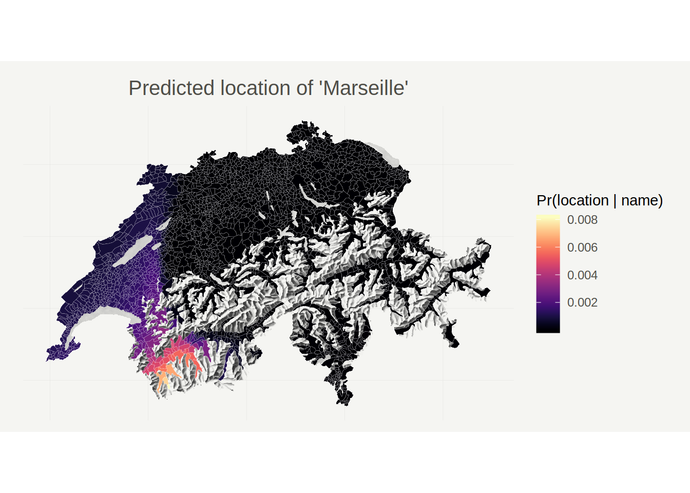
Apparently, Marseille would most likely be located in the Lower Valais, a French speaking area in the upper Rhone valley (incidentally, the actual Marseille is located at the opposite end of the Rhone!). This particular map also clearly illustrates the language border between the French and German speaking parts of Switzerland.
Finally, let’s see whether the model is also able to place a Romansh sounding name. I don’t know much Romansh, so I’m going to predict the location of an imaginary place called ‘Tuorta da Nuschs’ (Grisons nut pastry, a specialty local to the region).
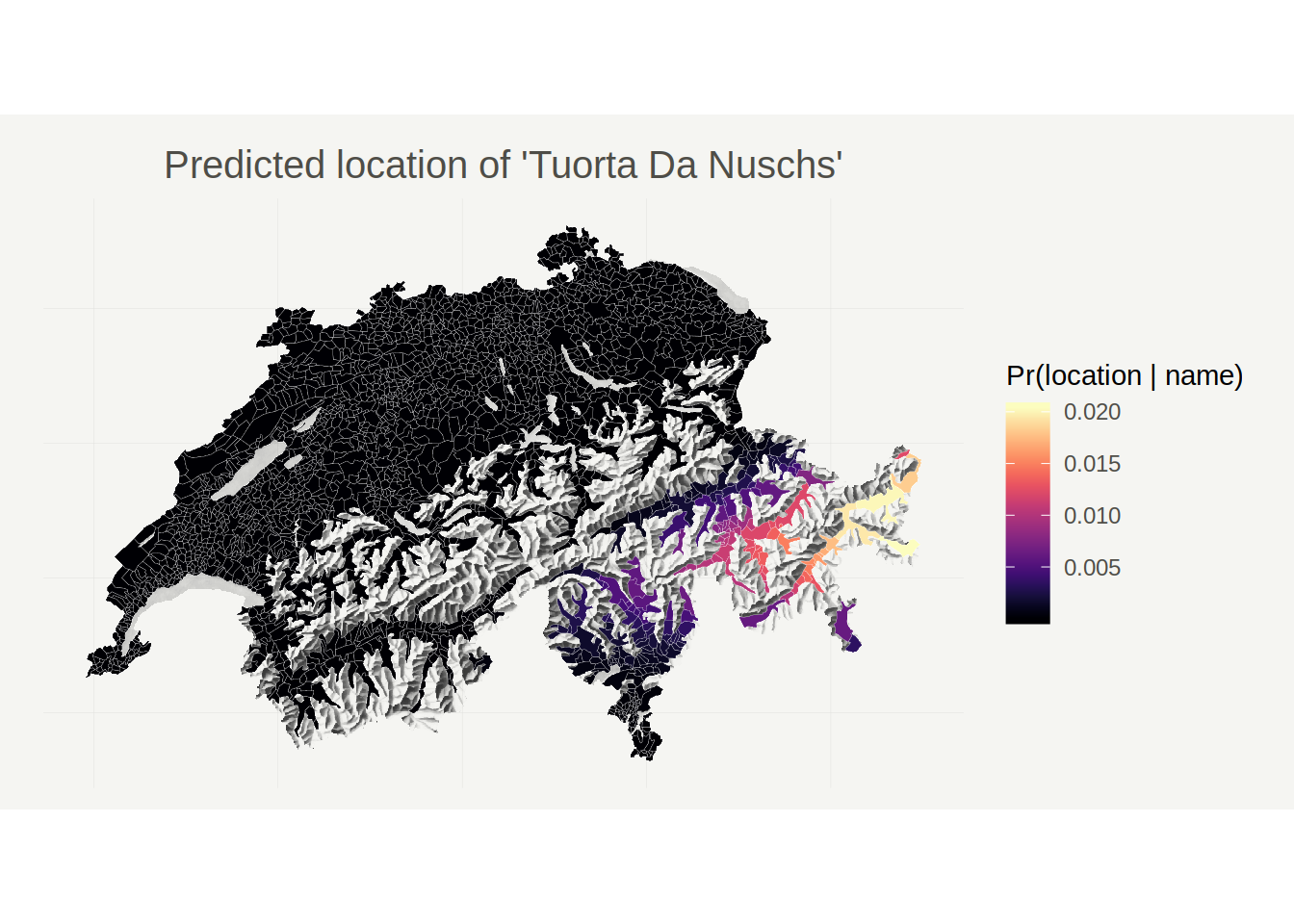
Again, the prediction is surprisingly plausible. The ‘Tuorta da Nuschs’ is a specialty from the Engadin valley, which is the area for which we get the highest predicted probabilities.
Detecting toponymic borders
The last question we had was whether it is possible to detect ‘toponymic regions’ and the borders between them. One way to address this question is to analyze distances between name distributions. Specifically, we could say that location \(i\) and location \(j\) are proximate in the ‘toponym-space’ if \(Pr(name \ | \ location_i)\) and \(Pr(name \ | \ location_j)\) are similar, and vice-versa. The key question then becomes: how should we measure the similarity of (name) distributions?
Fortunately, this is a very well researched question. There are many many ways to measure distances between distributions. For this project, I use the Hellinger Distance. For two discrete probability distributions with PMFs q(x) and p(x) and common support \(k \in K\) the Hellinger distance is defined as
\[ H(p, q) = \frac{1}{\sqrt{2}} \sqrt{\sum_{k \in K} \left(\sqrt{q(k)} - \sqrt{p(k)}\right)^2} \]
Unlike some other types of statistical distances, the Hellinger distance is a bounded metric, which means it has some properties that aid interpretation:
- It is bounded between zero (\(p\) and \(q\) are equal) and one (all events occur deterministically either under \(q\) or \(p\), but not both).
- It is symmetric, \(H(p, q) = H(q, p)\).
Computing the Hellinger distance between two discrete probability distributions requires summing over the entire support of the distributions. In our case, this would mean taking the sum over all \(39^{16}\) possible names of 16 characters, which is impossible. For this reason, I use an approximation: I compute the Hellinger distance only over a high-probability subset of the full support, namely over a random sample of 250 actually observed place names. To ensure that the Hellinger distance is still bounded between zero and one, I normalize the probabilities \(q(k)\) and \(p(k)\) so that they sum to unity despite sampling. More precisely, if \(K^S\) is the set of randomly sampled names I use as a proxy for the full support, I compute:
\[ \begin{align} H(p, q) & \approx \frac{1}{\sqrt{2}} \sqrt{\sum_{k \in K^S} \left(\sqrt{q'(k)} - \sqrt{p'(k)}\right)^2} \\ p'(k) & = p(k) / \sum_{k \in K^S} p(k) \\ q'(k) & = q(k) / \sum_{k \in K^S} q(k) \end{align} \]
With this formula at hand, we can compute the distributional distance between any two locations. Because we’re interested in detecting ‘borders’, I focus on instances where name distributions change rapidly over relatively small distances. In particular, using the same municipality datset as above, I first compute the approximate Hellinger distance between all adjacent pairs of municipalities, and then compute - for each municipality - the average Hellinger distance between it and its neighbors. This quantity should be high for municipalities that are on a toponymic border, i.e., that have a very different name distribution compared to their neighbors. The following map visualizes the results:
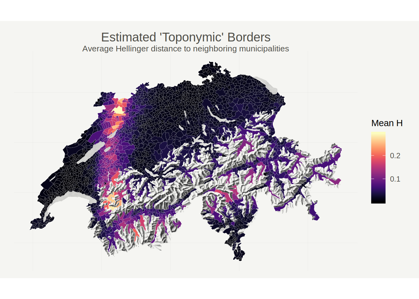
This map reveils two main borders: An east-west border that coincides almost exactly with the Röstigraben - the boundary between the German and French speaking parts of Switzernald; and a somewhat more fuzzy north-south border that separates the Italian speaking canton of Ticino and the trilingual Graubünden from the German speaking part of the country.
Concluding remarks
At this point the conclusion is clear: the (Swiss) toponym distribution is extremely learnable, even with relatively simple methods. More generally, I also think that this post shows that toponym data lend themselves to being analyzed with NLP. They’re abundant, and they contain an incredible amount of linguistic, historical, and anthropological information that is waiting to be explored.